Dense Model Serving on AWS EKS with Triton, vLLM, and GPU slicing

Introduction

In production MLOps, it is common to encounter a mismatch between hardware and workloads. We deal with monolithic, expensive GPU resources that are often overkill for a single small model, yet insufficient for the largest LLMs. This leads to the outcome where the infrastructure is either the bottleneck, or it is burning money on idle compute cycles.

Not everyone has infinite budgets to throw at their next AI adventure, so if there is some space left on that expensive H100 GPU, why not use it for something useful?

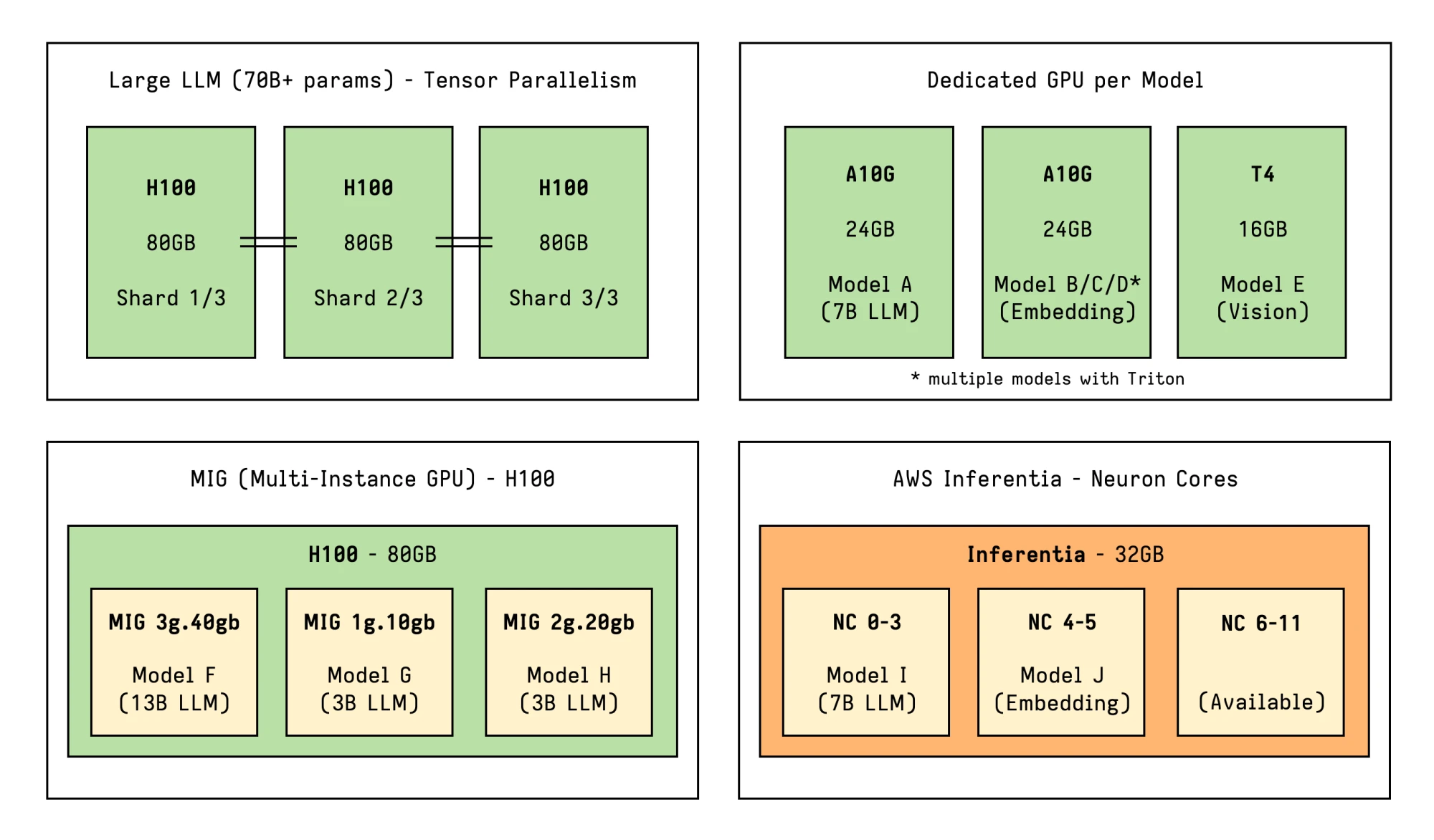
The objective is to achieve high-density GPU serving: we want to intelligently pack multiple smaller models onto a single GPU, while distributing the massive ones across multiple GPUs via Tensor Parallelism.

In this post, we will explore multiple technologies which can be combined allowing us to architect flexible model serving solutions on Amazon EKS:

• Karpenter for just-in-time GPU provisioning that matches capacity to demand
• Triton Inference Server for allowing heterogeneous models and software multiplexing
• vLLM for its memory-efficient model serving and LLM optimizations
• NVIDIA MIG, Time-Slicing and MPS for sharing GPU resources across smaller models
• Tensor Parallelism for scaling large models across multiple GPUs

If some of these technologies seem unfamiliar don’t worry, as they will be covered in the following sections. GPU slicing and sharing strategies specifically are covered with more detail in Appendix A.

This post will be mostly useful as an overview about all the different layers and components involved in a basic but versatile ML/LLMOps setup, to help while architecting your own solution.

Main Architecture (Amazon EKS)

The solution leverages Amazon EKS as the orchestration layer, which provides a managed Kubernetes environment without the operational overhead of managing the control plane, and integrates seamlessly with other AWS services like EC2 for provisioning vast amounts of diverse compute resources.

Plugins and add-ons are used extensively to enable additional capabilities like just-in-time dynamic provisioning, persistent storage, GPU feature support and more.

For added flexibility, we use two categories of node pools to handle different workload patterns and operational needs: static node pools are prefect for pre-planned capacity and slicing of big GPUs, while a dynamic pool managed by Karpenter is optimal for flexible, on-demand provisioning.

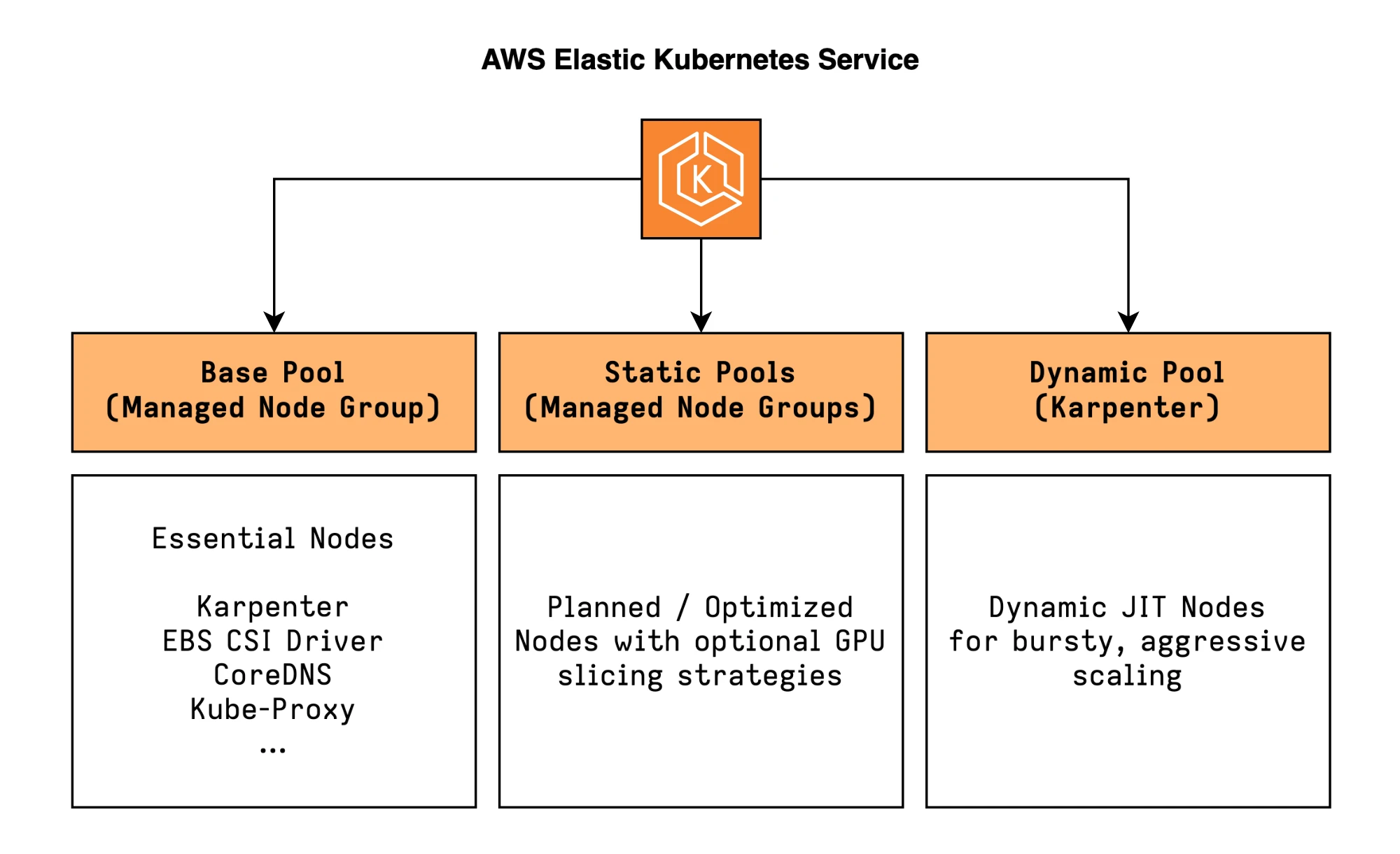
Besides these two pools, a general-purpose managed node group is used for running critical cluster components and add-ons, like Karpenter itself.

Static Pools (Managed Node Groups)

The static pools are ideal for steady workloads, where a strict budget is imposed, and most importantly where we want to optimize utilization by sharing the GPUs.

These pools use AWS Managed Node Groups rather than Karpenter, because the ecosystem is not yet mature enough to dynamically provision and manage sliced (e.g. MIG) instances. Some challenges are described in this document by NVIDIA and also related to Dynamic Resource Allocation (DRA) in Kubernetes and Karpenter.

The nodes will be labeled so that they can be targeted specifically during scheduling:

Labels:
  platform/node-type: gpu
  platform/gpu-sharing: mig # or "time-slicing" or "mps" or "none"

Dynamic Pool (Karpenter)

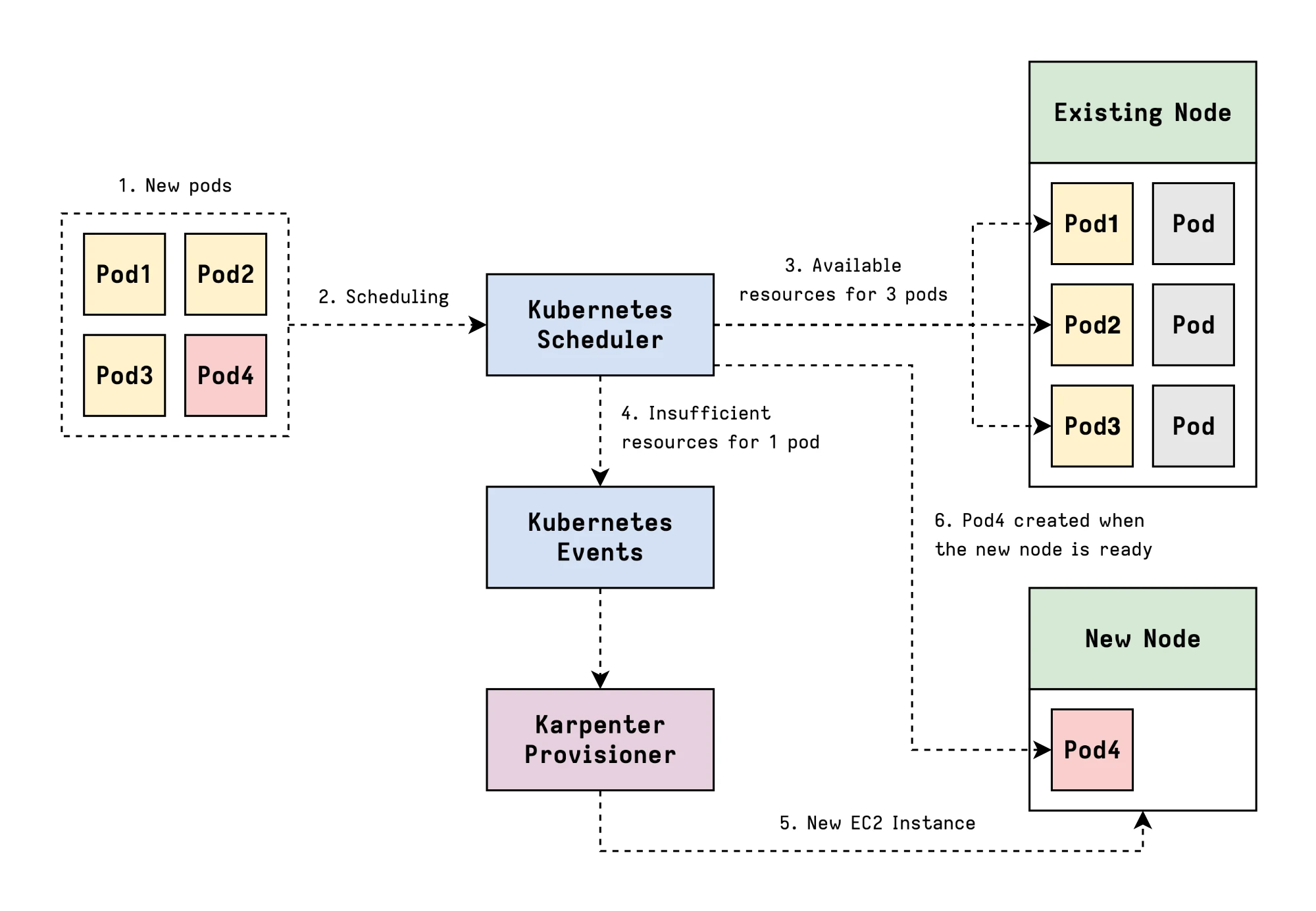
The dynamic pool is managed entirely by Karpenter. Unlike traditional autoscaling, which adds or removes nodes from predefined Node Groups, Karpenter dynamically provisions and deprovisions nodes based on the actual resource requirements of pending pods.

This handles everything that does not require a static pool: larger models requiring full GPUs, bursty workloads or requiring aggressive scaling, experimental deployments.

Karpenter will provision exactly what you need when you need it, and consolidate or terminate nodes when the demand decreases, optimizing for cost efficiency.

Workload Node Routing

The routing between these two node pools is managed through standard Kubernetes primitives.

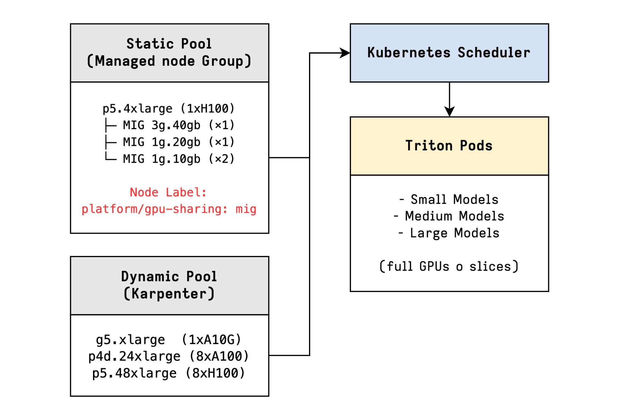
Pods that request specific GPU sharing resources (like nvidia.com/mig-1g.5gb for MIG) and include the appropriate node selector or affinity rules, will be scheduled onto the appropriate static pool.

nodeSelector:
  platform/gpu-sharing: mig

All other pods will be handled by Karpenter in the dynamic pool.

Be aware that mixing these two approaches in a single cluster requires careful planning, and a combination of selectors, affinities, taints and tolerations might be useful with more complex setups.

Essential Add-ons and Plugins

NVIDIA Device Plugin

The NVIDIA Device Plugin is the bridge between Kubernetes and NVIDIA GPUs. It’s a DaemonSet which runs on every GPU-enabled node and exposes the number of available GPUs and their capabilities to the Kubernetes scheduler.

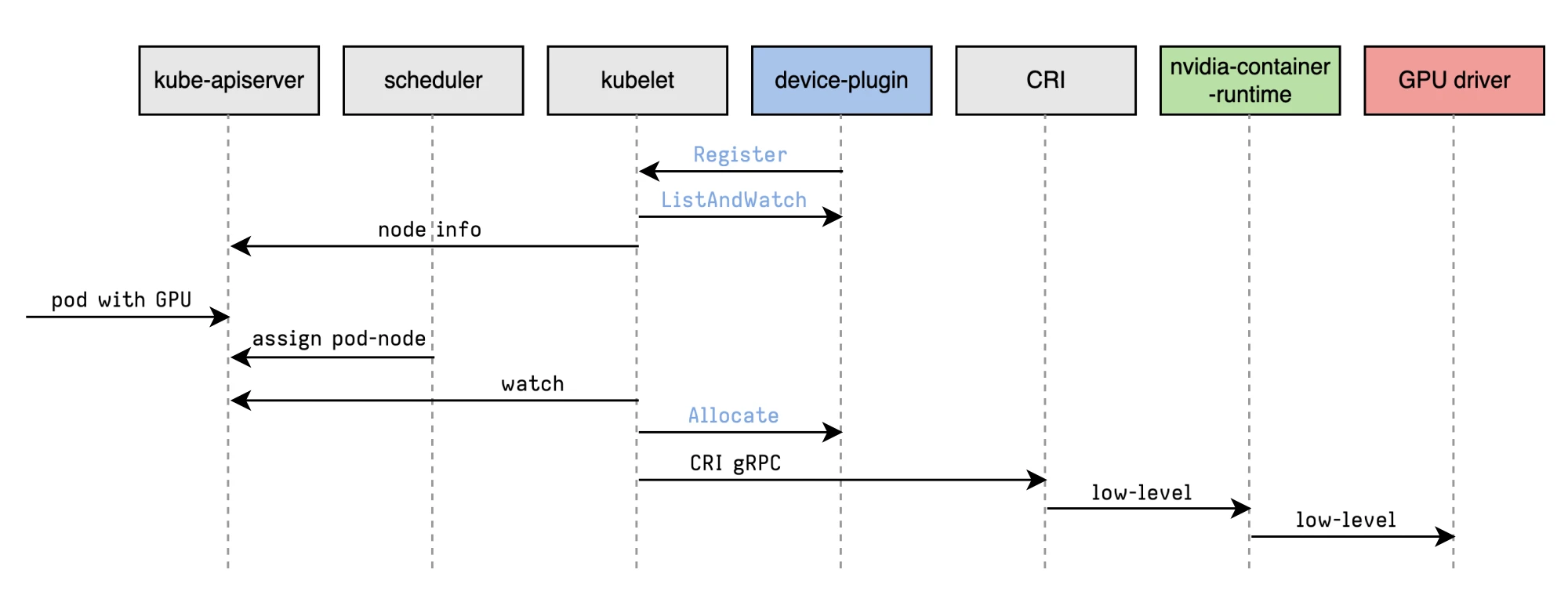
Original diagram by: Rifewang

With the daemonset deployed, NVIDIA GPUs can then be requested using the nvidia.com/gpu resource:

apiVersion: v1
kind: Pod
metadata:
  name: gpu-pod
spec:
  restartPolicy: Never
  containers:
    - name: cuda-test
      image: nvcr.io/nvidia/k8s/cuda-sample:vectoradd-cuda12.5.0
      resources:
        limits:
          nvidia.com/gpu: 1 # requesting 1 GPU
  tolerations:
    - key: nvidia.com/gpu
      operator: Exists
      effect: NoSchedule

For being able to instead request MIG slices, it will be necessary to configure the MIG_STRATEGY in the NVIDIA Device Plugin, which will then be made available as nvidia.com/mig-<profile>.

It will also be possible to oversubscribe GPU resources through Time-Slicing and MPS. Time-Slicing can be applied in itself to MIG slices as well.

At this point, it might be useful to know how to apply those settings selectively to different nodes. This can be achieved by having multiple configurations which will be applied to nodes selectively based on the nvidia.com/device-plugin.config label.

# values.yaml
config:
  # Default config for nodes without specific label
  default: "default"
  # Nodes with label nvidia.com/device-plugin.config=mig will use mig cfg
  # Nodes with label nvidia.com/device-plugin.config=time-slicing will use time-slicing cfg
  map:
    default: |-
      version: v1
      flags:
        migStrategy: "none"
        failOnInitError: true
    mig: |-
      version: v1
      flags:
        migStrategy: "mixed"
        failOnInitError: true
    time-slicing: |-
      version: v1
      flags:
        migStrategy: "none"
        failOnInitError: true
      sharing:
        timeSlicing:
          renameByDefault: false # <resource-name>.shared
          failRequestsGreaterThanOne: false
          resources:
            - name: nvidia.com/gpu
              replicas: 10

# Tolerations to run on GPU nodes
tolerations:
  - key: nvidia.com/gpu
    operator: Exists
    effect: NoSchedule

# Enable GPU Feature Discovery
gfd:
  enabled: true

As an example, if the above time-slicing configuration would be applied to a node with 4 GPUs, the plugin would then be advertising 40 GPUs instead.

The plugin can be installed through helm:

helm upgrade -i nvdp nvdp/nvidia-device-plugin \
  -f values.yaml \
  --version=0.18.0 \
  --namespace nvidia-device-plugin \
  --create-namespace

And the nodes should be labeled with the appropriate config like nvidia.com/config=time-slicing.

For MIG, some nvidia-smi commands need to be executed to enable this feature and configuring the slicing setup (more on this in Appendix A).

Neuron Device Plugin

The Neuron setup is covered in a separate blog post here: Coming Soon…

Karpenter

Karpenter is the component which allows just-in-time provisioning of nodes by looking at the pending pods, analyzing their resource requirements and constraints, and then provisioning exactly the right instance types to satisfy those requirements.

It will also take care of consolidating existing nodes for cost optimization.

Other Addons

Other useful addons are:

• Observability Add-On: you can also look into NVIDIA’s DCGM (Data Center GPU Manager) for exporting additional metrics
• AWS Load Balancer Controller: for exposing services through an AWS Load Balancer, LiteLLM can also be a great way to centralize models access while exposing a single service

NVIDIA Triton Inference Server

Dynamo-Triton, previously known as NVIDIA Triton Inference Server, is an open-source platform for AI inference which supports the deployment, scaling and inference of AI models from multiple machine learning and deep learning frameworks like TensorRT, PyTorch, ONNX, and more.

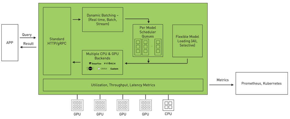
Diagram fron NVIDIA

The following are some of its key features in detail.

Dynamic Batching

Dynamic Batching improves the performance by automatically accumulating requests and batching them together before inferencing on the model. This usually results in better efficiency of GPU utilization, as many models have a strong imbalance between memory and compute requirements, and dramatic throughput improvements at scale.

dynamic_batching {
  preferred_batch_size: [ 8, 16 ]
  max_queue_delay_microseconds: 20000
}

A configuration like this one will try to batch requests into sizes of 8 or 16, but won’t wait more than 20ms.

Model Repository for Multiple Backends

Triton allows different Backends, which are wrapper around a specific ML framework. You might have PyTorch models for transformers, TensorRT models for optimized CNNs, portable ONNX models, and vLLM for serving LLMs. Without a unified serving layer, each framework would need its own deployment pipeline, monitoring setup, and operational tasks.

For more information about supported backends, see: Where can I find all the backends that are available for Triton?)

Triton’s Model Repository format is a simple file structure which greatly simplifies models management:

model_repository/
├── embedding-model/          # PyTorch
│   ├── 1/
│   │   └── model.pt
│   └── config.pbtxt
├── classification-model/     # TensorRT
│   ├── 1/
│   │   └── model.plan
│   └── config.pbtxt
├── llama-2-7b/               # vLLM
│   ├── 1/
│   │   └── model.json
│   └── config.pbtxt
└── object-detection/         # ONNX
    ├── 1/
    │   └── model.onnx
    └── config.pbtxt

• The root model_repository contains one or more subdirectories, each representing a different model.
• Within the model directory, there are version directories (1/, 2/) to allow multiple versions of the same model. This contains the actual model files.
• For each model, a config.pbtxt file defines its backend and configuration.

// Example model.json file for llama3-8b-instruct
{
  "model": "meta-llama/Meta-Llama-3-8B-Instruct",
  "gpu_memory_utilization": 0.8,
  "tensor_parallel_size": 2,
  "trust_remote_code": true,
  "disable_log_requests": true,
  "enforce_eager": true,
  "max_model_len": 2048
}

Triton will load all of the models exposing them through a common HTTP and gRPC API. Clients don’t need to know which backend serves each model, but they just make requests to /v2/models/{model_name}/...

Concurrent execution is handled depending by the different Scheduler configurations.

Concurrent Model Execution

Triton allows to serve multiple models and/or multiple instances of the same model on the same hardware.

# model0 partial config.pbtxt
instance_group [
  {
    count: 1
    kind: KIND_GPU
    gpus: [ 0 ]
  }
]

# model1 partial config.pbtxt
instance_group [
  {
    count: 3
    kind: KIND_GPU
    gpus: [ 0 ]
  }
]

The instance-group configuration allows each model to specify how many parallel executions should be allowed. Each parallel execution is referred to as an Instance.

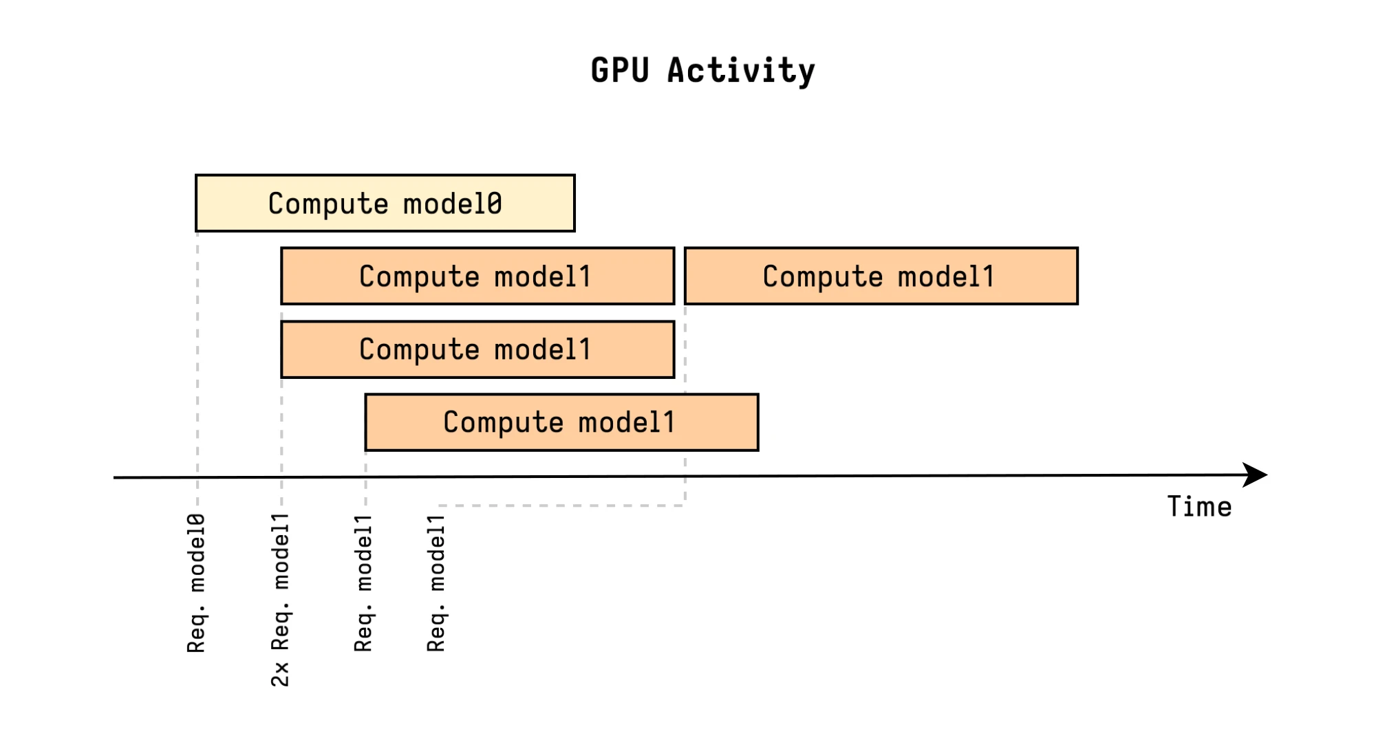
In this example, the first three model1 requests are immediately executed in parallel, while the fourth model1 one must wait for a free slot.

vLLM Integration

The vLLM engine is specialized for memory efficiency (LLMs are some of the models which require the most memory), high throughput, and low latency. By combining it with Triton, we can get both excellent performance and streamlined operations.

PagedAttention for Memory Efficiency

Even though this is not 100% accurate today, Paged Attention is a key optimization of vLLM, introduced by its popular paper Efficient Memory Management for Large Language Model Serving with PagedAttention.

Large language model inference has a memory problem. When generating text, the model needs to maintain a key-value (KV) cache for all previous tokens in the sequence. Even for a small LLM with average context lenght, this cache could easily consume dozens GB of memory per request. With traditional memory allocation, the cache is stored in contiguous memory blocks, leading to fragmentation and inefficiency.

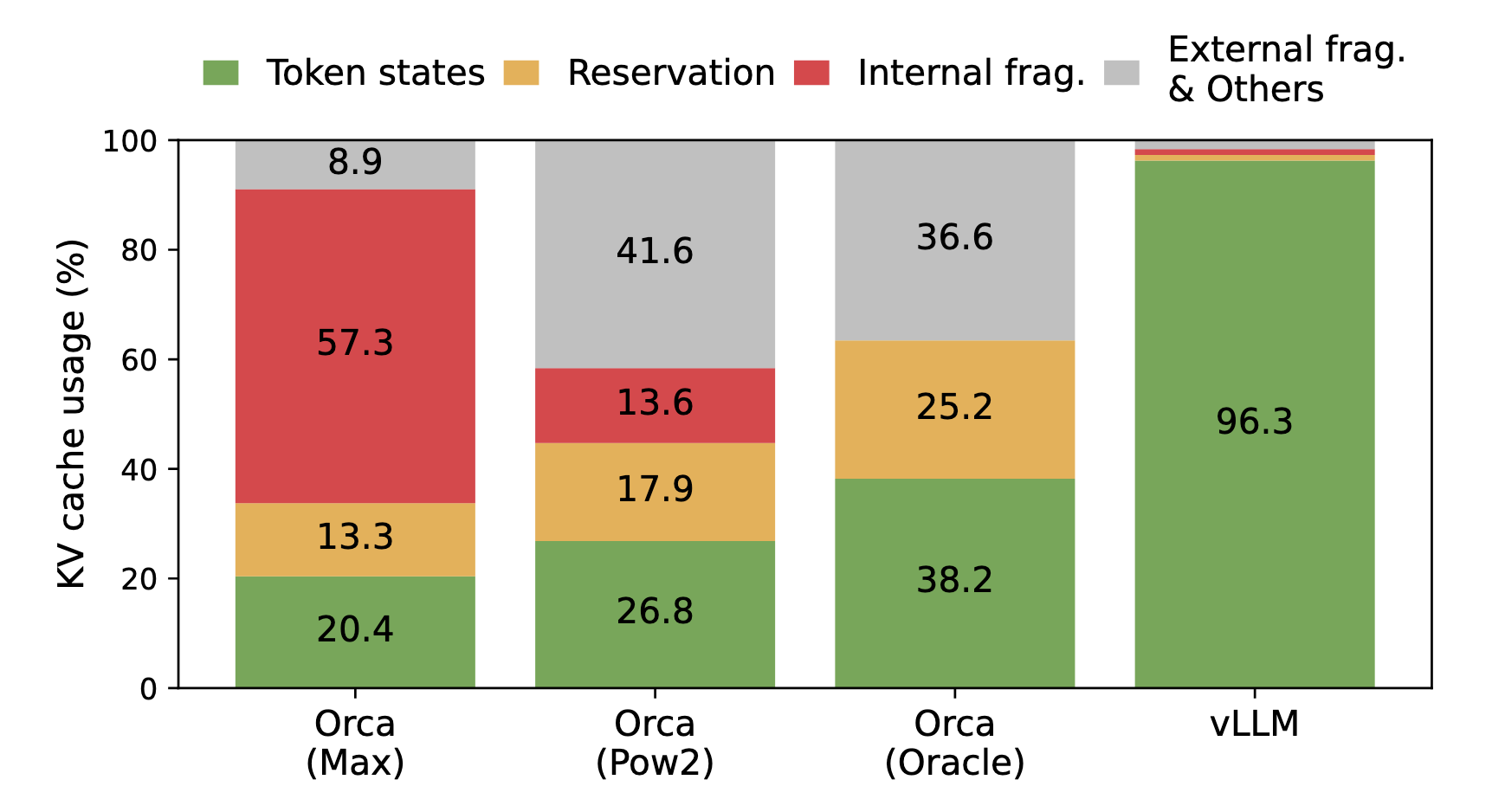
Average percentage of memory wastes in different LLM serving systems from the original paper.

vLLM solved this issue with PagedAttention. The core insight is to apply virtual memory concepts from operating systems to KV cache management.

Instead of allocating large contiguous blocks, vLLM divides the KV cache into small fixed-size pages. A request’s KV cache is then represented as a “page table”, mapping logical pages to physical memory locations.

This allows to either increase performance through more concurrent requests with the same memory footprint, or decreasing memory usage to enable serving of more models on the same GPU.

Appendix A: GPU Slicing and Sharing Strategies

NVIDIA Multi-Instance GPU (MIG)

Multi-Instance GPU (MIG) is an hardware feature available on higher-end GPUs like the A100 and H100, which allows the physical GPU to be partitioned into multiple instances.

MIG Diagram from NVIDIA

Each instance has dedicated memory, compute resources, and memory bandwidth, providing true hardware-level isolation. This means that multiple workloads can run simultaneously without interfering with each other, with predictable performance and fault isolation.

At the hardware level, an GPU like the A100 consists of multiple streaming multiprocessors (SMs), memory controllers, and memory slices. MIG allows to map subsets of these resources into discrete instances.

By default, MIG mode is not enabled, and it can be enabled on all GPUs on a specific GPU by running:

# Enable MIG mode on GPU 0
$ sudo nvidia-smi -i 0 -mig 1
Enabled MIG Mode for GPU 00000000:36:00.0
All done.

$ nvidia-smi -i 0 --query-gpu=pci.bus_id,mig.mode.current --format=csv
pci.bus_id, mig.mode.current
00000000:36:00.0, Enabled

If you do not specify a GPU ID, the MIG mode is applied to all the GPUs on the system.

The NVIDIA driver provides a list of profiles available for the MIG feature, which are the sizes and capabilities of the GPU instances that can be created.

# Example output for A100 80GB
$ nvidia-smi mig -i 0 -lgip
+-------------------------------------------------------------------------------+
| GPU instance profiles:                                                        |
| GPU   Name               ID    Instances   Memory     P2P    SM    DEC   ENC  |
|                                Free/Total   GiB              CE    JPEG  OFA  |
|===============================================================================|
|   0  MIG 1g.10gb         19     7/7        9.50       No     14     0     0   |
+-------------------------------------------------------------------------------+
|   0  MIG 1g.10gb+me      20     1/1        9.50       No     14     1     0   |
+-------------------------------------------------------------------------------+
|   0  MIG 1g.20gb         15     4/4        19.50      No     14     1     0   |
+-------------------------------------------------------------------------------+
|   0  MIG 2g.20gb         14     3/3        19.50      No     28     1     0   |
+-------------------------------------------------------------------------------+
|   0  MIG 3g.40gb          9     2/2        39.25      No     42     2     0   |
+-------------------------------------------------------------------------------+
|   0  MIG 4g.40gb          5     1/1        39.25      No     56     2     0   |
+-------------------------------------------------------------------------------+
|   0  MIG 7g.80gb          0     1/1        79.00      No     98     5     0   |
+-------------------------------------------------------------------------------+

The first number in the canonical MIG profile name indicates the compute capability (in terms of number of Streaming Multiprocessors), while the second number indicates the memory size in GB.

To create MIG instances, it is possible to use a command similar to this:

# Create MIG instances manually
sudo nvidia-smi mig -cgi 1g.5gb,1g.5gb,2g.10gb,2g.10gb,3g.20gb,3g.20gb -C

In case of EKS, the commands can be added as a bootstrap script to the node group user data, and once the node is ready, the NVIDIA Device Plugin will detect and advertise the MIG slices if configured properly:

kubectl get node <gpu_mig_node> -o json | jq '.status.allocatable'

"nvidia.com/mig-1g.5gb": "2",
"nvidia.com/mig-2g.10gb": "2",
...

Each MIG profile will be exposed as a separate resource which can be requested in the pod spec.

This strategy is ideal for workloads with predictable resource requirements, where smaller models can fit into MIG slices, and isolation between workloads is desired. It can also be useful for development and staging environments.

Time-Slicing

When using time-slicing, CUDA time-slicing is used to allow workloads on the same GPU to interleave with each other. However, there is no isolation whatsoever.

From a Kubernetes perspective, time-slicing is implemented by telling the device plugin to advertise more GPU resources than physically exist. If you have one physical GPU and configure 4 replicas, the plugin advertises 4 GPUs to Kubernetes. When 4 pods each request 1 GPU, they all get scheduled on the same physical GPU, and the driver handles time-slicing.

Time-slicing is also compatible with MIG, so it is possible to oversubscribe MIG slices as well.

This strategy is ideal for workloads with variable or bursty resource requirements, where multiple smaller models can share the same GPU without strict isolation needs.

MPS (Multi-Process Service)

MPS is an NVIDIA technology that allows multiple CUDA applications to share a single GPU context without significant context-switching overhead. In contrast to time-slicing, MPS does space partitioning and allows memory and compute resources to be explicitly partitioned while enforcing these limits per workload.

In Kubernetes, the device plugin will advertise multiple GPUs similar to time-slicing, so it will be possible to oversubscribe the physical GPU.

This strategy is usefule for workloads that require better performance isolation than time-slicing, and can be used on GPUs that do not support MIG.

Tensor Parallelism

Tensor parallelism addresses the opposite problem from slicing: what do you do when a model is too large for a single GPU?

There are multiple approaches to this, the most common one being layer-wise (pipeline) parallelism where each transformer layer is split across GPUs. For a 70B model with 80 layers, you could assign 20 layers to each GPU. During a forward pass, data would flow sequentially through each one:

• Input → [GPU 0: Layers 0-19] → [GPU 1: Layers 20-39] → [GPU 2: Layers 40-59] → [GPU 3: Layers 60-79] → Output

AWS Neuron for Inferentia/Trainium

Sharing of Neuron devices is covered in a separate blog post here: Coming Soon…